Chapter 3 File types and how to work with them in YASARA
3.1 Common model file types
YASARA loads numerous types of files, however we will limit our discussion to just three: .pdb, .yob, and .sce. These file types are the most capable and easiest to export to other programs.
Information on the other file types that YASARA can work with can be found using the SearchDoc command.
3.1.1 .pdb files
.pdb formatted files are the gold standard for recording the three dimensional structures of biomolecules. Most visualization programs take .pdb files and many structural analysis methods start with a .pdb file or data generated from a .pdb file. Moreover, the Research Collaboratory for Structural Bioinformatics or RCSB or Protein Databank stores the structural information on the >100,000 biomolecules in the database in .pdb format. Therefore, the first files you should know how to use are .pdb files.
A .pdb file consists of a few parts shown in Figure 3.1. A .pdb file can be viewed in a plain text editor such as TextEdit or NotePad and reveals that it consists largely of the atom identifiers, the coordinates for each atom in the molecule, the temperature or B-factor and the header.
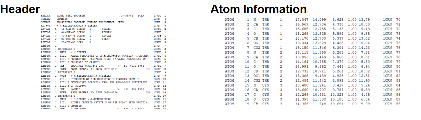
Figure 3.1: The PDB file format
.pdb files are easy to move across several programs but are limited in that they contain only location information and the reliability of those locations. Any manipulations that are performed to color or stylize the molecule are not included.
3.1.2 .yob files (YASARA object)
Like .pdb files, .yob files contain the 3-D coordinates for each atom, but also contain style information. If a color for a particular residue is set to red, it will be red in the saved .yob file as well. This file format is useful for annotating molecules and keep these annotations to pick up again later (keep a notebook to help remember what it all means though!). A .yob file can only contain one Object from the Scene Content table however. If you want multiple Objects or to save everything you need a Scene file.
3.1.3 .sce files (Scene files)
.sce files are the most sophisticated file type in YASARA. A scene file can contain 3-D data and stylization on multiple objects. This can also include any labels (5.2), colors (4.3), and other manipulations you may perform.
With more content, comes a need to be careful to keep track of the information effectively. So use .sce files for key models or findings and use .yob or .pdb files for intermediate steps.
3.2 Starting to work with models in YASARA
So far, I have shown you what YASARA can tell you and how to find information but we have not yet worked with any models. From this section forward we will be fully immersed in using YASARA. I encourage you to follow along and try to recreate each step that I do. Then test your understanding with the end of chapter exercises.
3.3 Loading a model
Model files can be loaded into YASARA from the local hardrive or retrieved from the RCSB server.
3.3.1 .pdb files
Files stored on the hard drive can be loaded by:
File > Load > PDB file, then navigate to the file location.
OR
# Specify LoadPDB, then put the name of the file. This assumes the file is in the pdb folder within the YASARA file tree or in the working directory
>LoadPDB <<PDB:ID>>


# Example that should work as 1crn is provided with the YASARA software
>LoadPDB 1crn
OR
Drag the file into an empty YASARA window
3.3.2 Getting a .pdb file from the internet
Files stored on the hard drive can be loaded by:
File > Load > PDB file from Internet, then provide the PDB ID (ex. 1UBQ) in the dialog box that appears.
OR
# Specify LoadPDB, then put the name of the file. This assumes the file is in the pdb folder within the YASARA file tree or in the working directory
>LoadPDB <<PDB:ID>>, download=yes


# Example that should work as 1crn is provided with the YASARA software
>LoadPDB 1crn, download=yes
Note that the only difference in the commands is adding download = yes. Also realize that you can download the files directly from the RCSB via the linked form or from the individual page for the model using the download button.
3.3.3 .yob files
Files stored on the hard drive can be loaded by:
File > Load > YASARA Object, then navigate to the file location.
OR
# Specify LoadYOb, then put the name of the file. This assumes the file is in the yob folder within the YASARA file tree or in the working directory
>LoadYOb filepath/file.yob

# Example that should work as dopc is provided with the YASARA software
>LoadYOb yob/dopc
OR
Drag the file into an empty YASARA window
3.3.4 .sce files
Loading a scene file will replace and delete anything else that was in the window beforehand. You can add .pdb or .yob files to Scene files, but you cannot add a Scene file to a .pdb or .yob.
Files stored on the hard drive can be loaded by:
File > Load > YASARA Scene, then navigate to the file location.
OR
# Specify LoadPDB, then put the name of the file. This assumes the file is in the yob folder within the YASARA file tree or in the working directory
>LoadSceb filepath\file.sce

# Example that should work as dhfr_water.sce is provided with the YASARA software
>LoadSce sce\dhfr_water.sce,Settings=No
OR
Drag the file into an empty YASARA window
3.4 What does Obj vs. Mol vs. Res vs. Atom mean?
YASARA organizes models at several levels, which permits easier control of manipulations to the model. In the simplest sense, an Object consists of one or more Mol (Molecules) which consists of one or more Res (Residues) which consist of one or more Atoms. Let’s unpack each level in a bit more detail before showing how this might be useful.
Obj (Objects) – Objs are the highest level of organization. An object is a complete model composed of one or more molecules. Objects can be split into several objects. Objects are typically numbered.
Mol (Molecule) – A Mol is the second level of organization and typically refers to a single contiguous chain within the scene. A Mol can be as simple as a single atom or a single amino acid or be larger and composed of several atoms or amino acids. Mol are defined in the .pdb or .yob file and can be broken into smaller pieces. Molecules are typically called “A” or “B” or another alphabetical name
Res (Residue) – A residue refers to a subunit of a Molecule. This name comes from classical biochemistry and an refer to a single saccharide within a longer chain, a single amino acid within a protein, or a single nucleotide within a nucleic acid. Residues are composed of one or more Atoms and typically are not split.
For most structural biochemistry, we think about residues and their function within the larger molecule. Residues are typically referred to by the three letter amino acid, nucleic acid, or carbohydrate name. Search the RCSB Ligand database if you do not recognize the abbreviation.
Atom – Atoms are the smallest unit within YASARA and describe single atoms. Atoms are not split in YASARA (no fission!). Atoms are referred to by their IUPAC names but can also be referred to in organic chemistry nomenclature (e.g. C or N ).
3.4.1 Why is the organization important?
Like the English language where sentences contain nouns and verbs, which define the action and who/what was involved, YASARA requires an action to perform and what to act on. The examples below in code chunk below give a few examples of how these commands work.
# Load a molecule into the window so that we can see the effects of each command
>LoadPDB 1crn

# Command examples to try
# Color all alanine residues red
>ColorRes ala, red

# Color Obj 1 blue
>ColorObj 1, blue

# Rotate Obj 1 around the y axis 1 degree
>RotateObj 1, Y = 30

# Count all the amino acids in Obj 1
>CountRes Obj 1 # the result of the count will appear on the same line as the command

# Show all the Hydrogen bonds in Molecule A
>ShowHBoMol A
The general YASARA syntax or grammar for commands, is ActionLevel and then the specifics of the molecule or part of the molecule to affect. Most commands can be used at any level so:
# Same action different levels
>ColorObj 1, red

>ColorMol A, red

>ColorRes 1, red

>ColorAtom 1, red
Effectively there are 4 nouns and lots of verbs. So if you can remember the levels of organization and the basic verbs, you can manipulate and analyze most any model.
3.5 Building a molecule
In addition to loading existing models, you can construct your own models using a variety of methods. If you are going to use the Build command to make a molecule such as a protein or cholesterol, you will need a set of instructions such as the protein sequence in FASTA format or the SMILES string. The sequence can be found in databases such as Uniprot under “Sequence’ or Ensembl. The SMILES string can be found in Section 4 of the Pubchem page. Examples of building various atoms and molecules are shown in the code chunk below.
# Build a sodium atom
>BuildAtom Na

# Build an amino acid, lysine in this case
>BuildRes lys

# Build maltotetraose from a SMILES string
# Results of this command are shown in Figure 4.2
BuildSMILES String="C(C1C(C(C(C(O1)OC2C(OC(C(C2O)O)OC3C(OC(C(C3O)O)OC4C(OC(C(C4O)O)O)CO)CO)CO)O)O)O)O"

# Build a molecule from a fasta file
# Results of this command are shown in Figure 4.2
>BuildMol C:path\to\file\testprot.FASTA
The Build command can be used to make a single atom, an amino acid, or a molecule. Realize the Build command will simply make the molecule and it does not “fix” it to make it accurate in any way as shown in Figure 3.2. Thus molecules made from this method will likely need energy minimization or see section ??.
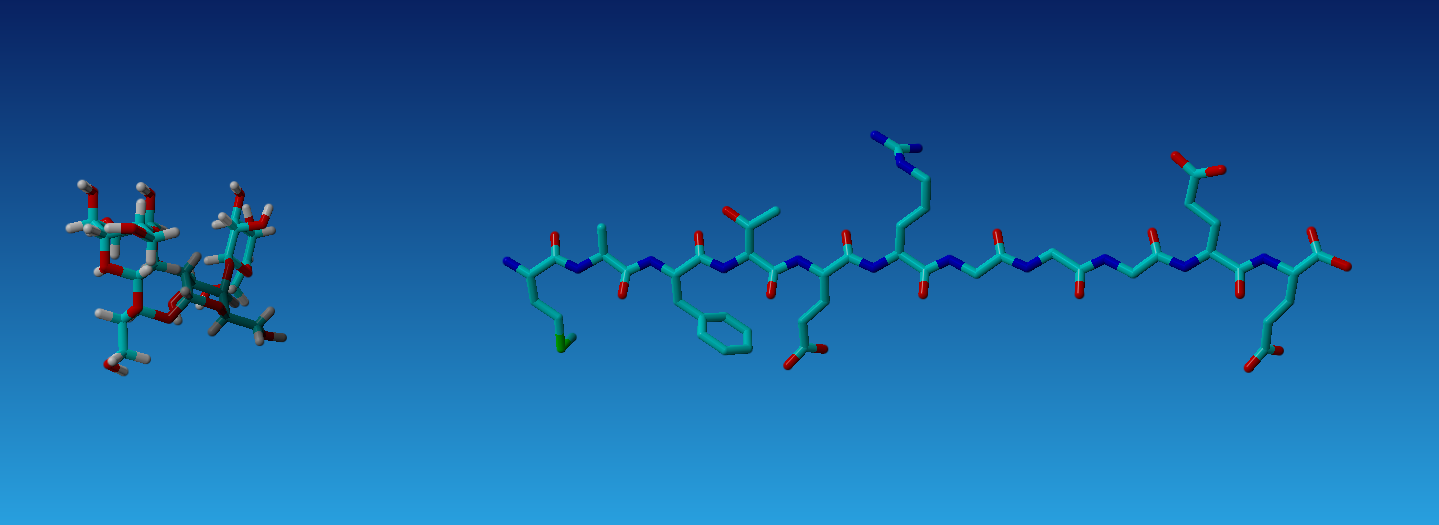
Figure 3.2: Results from using the BuildMol from a SMILES string and from a FASTA file of protein sequence
3.6 Saving Models
Once you have your model or scene in a form that is useful, you can also export the data. This is the one action I typically prefer to use the GUI over the command line, however I will show the command line method as well. Additionally, saving via the GUI has one trick, so I will show you how to do this in pictures as well (For example: 3.3).
Remember, there are some advantages and disadvantages to each file type so review the section on file formats (3.1) if you are uncertain about which format to use.
3.6.1 .pdb files
File>Save As>PDB file, then pick your Obj(s) and click OK, then select your file name and destination and click OK.
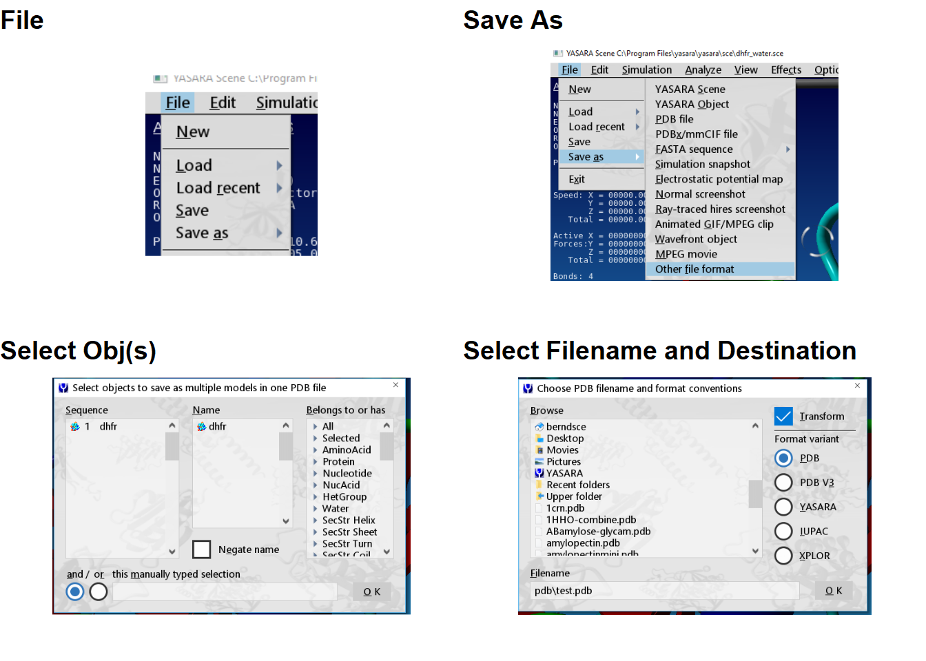
Figure 3.3: Saving a PDB file using the GUI
You will note that the first menu in 3.3 where you select Obj(s) has a selection bar at the bottom which you can enter text. This is not the filename, this is for you to pick a Molecule name or atom numbers. The file name goes in the second menu. Sometimes there will be a asterisk before .pdb (*.pdb) in the Filename box. This is a placeholder which you replace with your filename.
# Command then which Obj(s) have the source model,
# then the file name in this case test.pdb and some arguments
>SavePDB 1,pdb\test.pdb,Format=PDB,Transform=Yes
It is possible to save several Objects or Molecules in the same PDB file, but you will likely need to Transfer them all to the same set of coordinates first. Transfer is found in the Edit menu.
3.6.2 .yob files
Saving a .yob file is very similar to saving a pdb file, only without the issues of coordinates.
File>Save As>YASARA YOb, then pick your Obj, file name, destination, and then click OK.
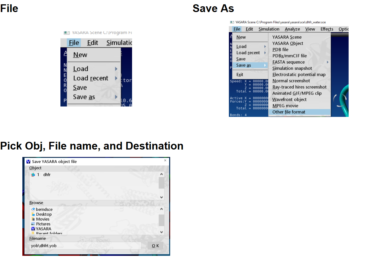
Figure 3.4: Saving a file in .yob format using the GUI
# Command then which Obj(s) have the source model,
# then the file name in this case dhfrt.yob
>SaveYOb 1,yob\dhfrt.yob
A .yob can only contain one Object, if you need to save more than one object in a single file, use .pdb or .sce.
3.6.3 .sce files
Saving a model as a .sce file is the simplest of all the file types as it save everything in the viewing window.
File>Save As>YASARA Sce, then pick your file name and destination.
# Command then the file name in this case dhfr_watertest.sce
>SaveSce sce\dhfr_watertest.sce
3.7 Adding and Removing Objects
Once there is a model loaded into the scene, it is possible to remove one or more objects from the actions and analysis that are occuring. This is useful if you are doing comparisons of multiple objects or for some of the more advanced functions of YASARA covered later. If you are simply looking to make the model invisible, the Hide command covered in section 4.2.2 is more appropriate.
The commands to remove an object and bring it back are Remove and Add respectively. This command only works on objects. Notice that when you use Remove that the Object disappears from the screen and the Scene Content columns Act and Vis change to ‘No’ (2.1.2). When you remove an object, the object still is listed in the scene content and will be included in .sce files that are saved, but it is no longer affected by commands and is invisible until it is added back.
# Load 1UBQ from the RCSB
>LoadPDB 1ubq, download=yes

# Remove the object, in this case it is designated as 1
>RemoveObj 1

# Make the object active again
>AddObj 1
3.8 Clearing the scene
If you want to clear everything out of the scene and start with an empty workspace You need the Clear command. If you have unsaved work, you will be prompted to save this work or to delete everything without saving.
From the menu: File>New
From the command line:
#  Clear everything from the scene
>Clear
3.9 Knowledge Self-Checks4
If you had colored a molecule and wanted to save the model and the stylizing of the model, which file types would be best?
What does the asterisk (*) mean in the Filename box when loading or saving a file?
What is the largest level of model organization in YASARA? The smallest?
What repository contains most biomolecule models?
What might each of the commands below do? What do they act on?
>LoadPDB 1ubq, download=yes

>SelectAtom 100-150

>ColorObj 3 4, green

>CountAtom Obj 2 Ala