Chapter 5 Adding annotations to your scene
With the various manipulations covered in Chapter 4, we can now start making figures to display biomolecule structures. This chapter will cover the basics of annotation and conclude with some tips on making good figures (5.4). We will start with making a basic image of a protein and then add layers of annotation.
As a note, many of the annotations added here, can be added via standard illustration or photo manipulation software as well. Therefore, do not see this as the only way to make a figure using structural data, just one way.
5.1 Saving an image
The first step in making a figure is to know how to save an image of your model. Thus far, I have described how to save the model itself, but not how to take an image. There are two levels of image quality when saving, the standard screen shot and RayTrace. The latter is the preferred method however, the standard screen shot works in most cases (see 5.1.2 for caveat).
To save an image via the menu: File>Save As>Normal Screenshot, then choose your filename and destination.
For a raytraced image via the menu: File>Save As>Ray traced hisres screenshot, then set your options (5.1.3) and click OK, then select your destination and image dimensions and click OK.
# Load PDB file
>LoadPDB 1crn

# Save an image of the model in PNG format
>SavePNG png\test.png

# Saving a ray traced image in PNG format
>RayTrace png\test.png,X=1024,Y=00541,Zoom=1.0,Atoms=Balls,LabelShadow=No,SecAlpha=100,Display=Yes,Outline=0.0,Background=No
I don’t recommend saving images via the command line, especially ray traced images and all the options. The ability to alter the background texture and image size however are great advantages of using RayTrace over SavePNG.
5.1.1 Change the background color
The background color is changed via the ColorBG command followed by the color of choice. White is the typical value however it depends on your medium. You can also set the background to be a gradient between two colors.
To change the color via menus:
View>Color>Background, then select your color and click OK.
If you choosing a gradient, then click Continue with Bottom Color and then selecting a color and clicking OK. In the command line this appears as below.
# Color background a single color
>ColorBG green

# Color background as a two-color gradient
>ColorBG green, blue
5.1.2 Hide the HUD!
If you use the SavePNG command to take a normal screenshot, everything in the scene including the HUD will appear in the image. To hide the HUD, press the Insert key or type HUD off in the command line. This will save you having the text of the HUD appear and gives you more image space to occupy with your biomolecule.
5.1.3 Ray Tracing options
Ray tracing requires downloading POV-Ray from www.povray.org and installing it in the pov folder of YASARA. In some versions of YASARA, this can be done via menus by:
Help>Install>POVRay
More details of installing POV-Ray can be found by using SearchDoc for the command RayTrace. The page on the RayTrace command also describes all the options for ray tracing in detail and I will summarize the key ones here.
Transparent Background – When this box is checked or Background=No, then everything that is not model will be transparent. This is a great feature for when making images for articles or presentations as it saves cropping of the background out of the image later.
Label Shadow – If checked or set to Yes, then any labels that you add (see section 5.2), will have shadows. This is a neat effect for presentations, but not something I would use in a figure in a paper.
X and Y values – This is the size in pixels of the final output from the ray tracing. To make a high resolution image for a paper or article, I recommend increasing these values by 2 to 5-fold and then shrinking the image size after inserting it. This reduces the pixelation issue that haunts structural biologists. Increasing these values will make for a larger file size so do not go crazy.
5.2 Labels
Labels are useful for explicitly marking atoms, distances, molecules, and other aspects of the scene contents. Labels can be positioned freely once they are made and maintain their orientation to the viewer throughout rotations of the scene.
To add a label via the menus:
Effects>Label>Pick your option, then select what will be labeled and click OK, then define the label parameters (5.2.1) and then select the color OR click OK.
The command to add a label is Label followed by the level of organization or distance (Dis). There are a number of parameters to be set afterwards (see Section 5.2.1 for more details.
The code below shows how to make the image in Figure 5.1.
# Load PDB file
LoadPDB 1crn, download=yes

# Position the model for viewing and labeling
>PosOriObj 01, X=0.000, Y=0.000, Z=50.000, Alpha=-5, Beta=280, Gamma=-15

# Stylize the molecule and scene area
>ColorBG White
>Style Ribbon
>Style Sidechain=stick
>ColorObj 1, grey

# Color Arg 17 blue and show in Ball style
>ColorRes 17, blue
>BallRes 17

# Make a blue label showing Arg 17 and have it be to the right of the target
>LabelRes Arg 17,Format=RESNAME RESNUM,Height=2.0,Color=Blue,X=10.0,Y=-1,Z=0.0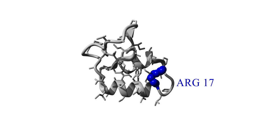
Figure 5.1: Resulting image of labeling code
5.2.1 Label parameters
Scene/Obj/Res/Mol/Atom/Distance – These options are under the Effects>Label menu. With the exception of Distance, all of them describe a level of organization. Distance will calculate the distance between the selection and display that number.
Format – This option describes what aspect will be labeled. RESNAME is the three letter code for the residue, RESNUM is the residue number. You can also put arbitrary text in this space.
Height – This defines how tall the text will be in Angstroms, which is 10-10 meters. This is really small compared to a human but is the standard unit of measurement for biomolecules. The text in Figure 5.1 is 2 angstroms tall for reference.
Color – Defines the color. Can be chosen using words or numbers as in section 4.3.
X, Y, Z – Indicates where the label is placed relative to the target of the label. The units are in angstroms. Placing the label is the trickest part of labeling part of a scene.
After you have created the label, if you want to move it to a new location, left-click on the label and you can freely move it around the screen using the mouse commands described in 4.1. This is very useful when making figures.
5.2.2 Removing a label
To remove a label, you can left-click on the label and press delete. Alternative use the command Unlabel. Typing UnlabelResAll removes all amino acid labels.
5.3 Adding Hydrogen Bonds
Hydrogen bonds are important weak interactions found throughout biochemistry. Hydrogen bonds hold \(\alpha\) helices together, connect \(\beta\) strands to form sheets, and can have dramatic effects on protein activity. Showing hydrogen bonds explicitly can show the role that these important interactions play in your biomolecule of interest.
In the scene we have created, it would be nice to show the role of Arg 17 in the structure of the protein. The side chain of the protein makes one or more hydrogen bonds with other parts of the protein so let’s show them. First you need to add hydrogens if they are not already in the molecule using the AddHyd command. Then use the ShowHBo along with your selection to show the hydrogen bonds.
From the menu:
View>Show Interactions>Hydrogen bonds of>Pick your option, then select your Obj/Mol/Res/Atom to show hydrogen bonds and then specify if you only want to show hydrogen bonds within your selection or all the hydrogen bonds that your selection makes. This is the Extend command shown in the code chunk below.
You can also add hydrogen bonds by selecting an atom and bringing up the pop-up menu. Within the pop-up menu choose Show>Hydrogen Bonds>Pick your option. The menu thereafter will relate to the Extend command described in the previous paragraph.
From the command line:
# Load PDB file
>LoadPDB 1crn, download=yes

# Position the model for viewing and labeling
>PosOriObj 01, X=0.000, Y=0.000, Z=50.000, Alpha=-5, Beta=280, Gamma=-15

# Stylize the molecule and scene area
>ColorBG White
>Style Ribbon
>Style Sidechain=stick
>ColorObj 1, grey

# Color Arg 17 blue and show in Ball style
>ColorRes 17, blue
>BallRes 17

# Make a blue label showing Arg 17 and have it be to the right of the target
>LabelRes 17,Format=RESNAME RESNUM,Height=2.0,Color=Blue,X=10.0,Y=-1,Z=0.0

# Add hydrogens to 1crn
>AddHyd all

# Add hydrogen bonds to Arg 17
>ShowHBoRes 17,Extend=Yes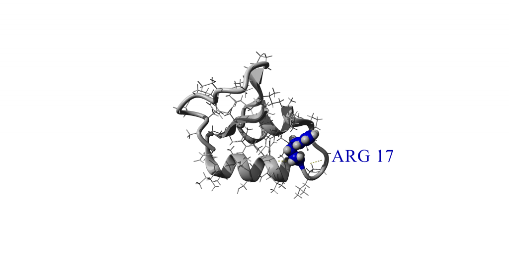
Figure 5.2: Resulting image of code adding hydrogen bonds to Arg 17
You will notice that 3 hydrogen bonds appear, although one is hidden by the side chain and requires rotation of the image to view.
5.3.1 Coloring hydrogen bonds
You can change the color of hydrogen bonds using the ColorHBo command as shown in the code chunk below. You must specify the color, the transparency (Alpha), and whether the bond inherits the color from the bounding atoms. This latter option is useful if you have certain hydrogen bound atoms colored the same and you want the bonds to be that same color.
From the menu:
View>Color>Hydrogen bonds, then select your color, transparency (alpha), and whether it inherits atom colors.
From the command line:
# Change hydrogen bond color to blue with 50% transparency and do not inherit atom colors
>ColorHBo Color=Blue,Alpha=50,Inherit=No
5.4 Making good figures
A good figure can convey more than the text ever could, while a bad figure can confuse the reader. Therefore it is important to keep a few considerations in mind when making figures of biomolecules. These ideas can apply to other types of figures and data but we are focused on biomolecule figures. Other tips on making figures can be found here. Additionally, a good illustration or graphics program is useful when combining figures. I recommend Inkscape or Google Drawings which is found within the Google Drive framework. Both are free and pretty easy to use.
5.4.1 Considerations when making a biomolecule figure
Why am I making the figure? – Don’t make a picture because you can, have a purpose and a point.
What am I trying to convey with this figure? – What are the two or three main ideas that the figure needs to convey. If upon making the figure, these aren’t obvious. Then further work is needed.
Don’t be messy – Remove unecessary parts of the molecule, try to crop the figure appropriately, and don’t go overboard. As in consideration #1, don’t show something because you can, show it because it matters.
Use labels, colors, and representations – This chapter has shown how to add annotations to figures, so use these to your advantage.
Make text legible – If you think the text is too small, then it probably is. If you think it is just right, then it is probably still too small. Claus Wilke’s excellent book on data visualization shows this principle very well.
Have a figure legend – Where possible use text to help the reader sort through the figure and the meaning.
Let’s look back at Figure 5.2 and you will notice that it violates principles 2, 3, 4, possibly 5 and 6. Now look at a revised figure (Figure 5.3). The unecessary side chains are gone and labels have been added to amino acids that interact with Arg 17. Additionally, the amino acids that are shown are colored by element with hydrogen bonds. So now we not only see the hydrogen bonds made by Arg 17, we also see the hydrogen bonding partners and the types of chemical groups involved. This figure still has an issue: the label for Arg 17 blocks the structure. Moving it away might confuse the reader, so why not save an image of the molecule and move to another program to add an arrow.
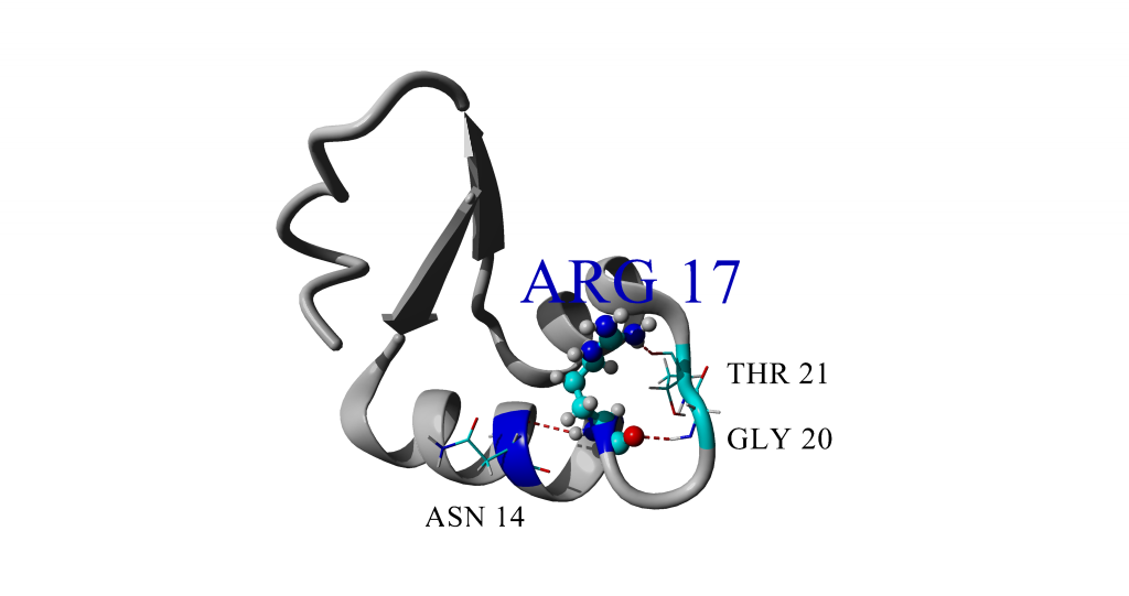
Figure 5.3: Better(?) figure of 1CRN showing interactions with Arg 17
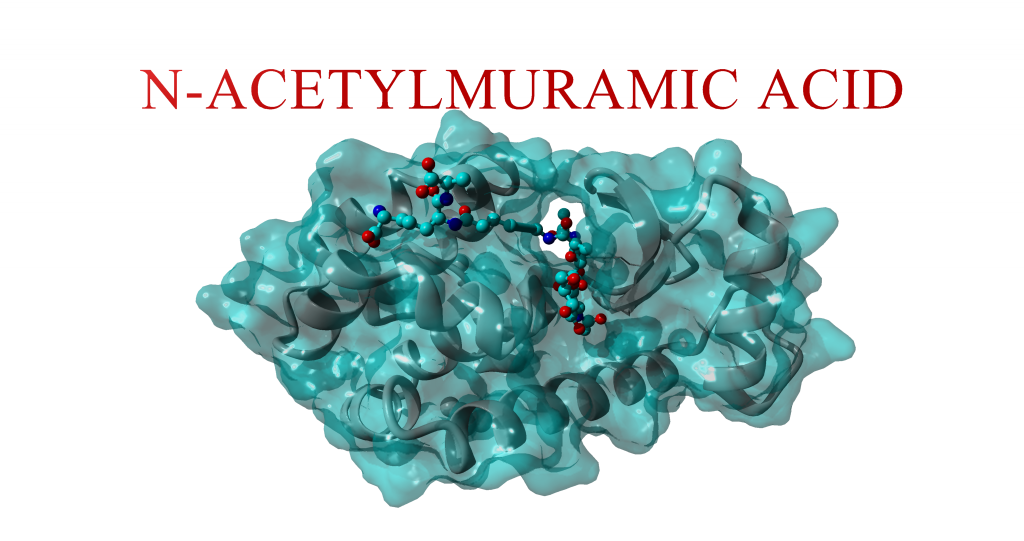
Figure 5.4 shows the figure after moving the Arg 17 label over and adding an arrow in Google Drawings to indicate what the label refers to. You will notice I left the size of the Arg 17 label larger and in blue compared to the other labels. This was intentional to help my reader focus on Arg 17. Also notice I made an informative figure legend.
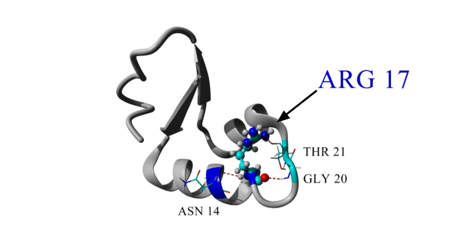
Figure 5.4: Model of structure 1crn showing how Arg 17 (shown by arrow in ball and stick representation) hydrogen bonds within the protein. Hydrogen bonds are shown as dotted red lines between donor and acceptor atoms. Amino acid side chains are colored by element with carbon colored cyan, nitrogen colored blue, oxygen colored red, and hydrogen colored grey.
If you are still struggling, show your figure to a peer or mentor and get feedback. I also recommend reading Fundamentals of Data Visualization by Claus Wilke to get a sense of best practices for other types of data. While not aimed at biomolecules, some of the principles and ideas in this book can help with figures in general.